41 excel chart labels from cells
Using a named range in VBA for chart data labels option explicit sub adddatalabelsfromcells () dim targetchart as chart dim labelrange as range set targetchart = activechart if typename (targetchart) <> "chart" then msgbox "select a chart, and try again!", vbexclamation exit sub end if set labelrange = worksheets ("linest").range ("mylabels") with targetchart.seriescollection (1) … Dynamic Chart Data Labels : excel Currently, my background is white, bar chart is red, data labels are white. For the most part this works fine. However, when a particular filter on the slicer is selected, one of the bar has a very small value and the data label exceeds the bar. Since the data label font is white and the background is white, im not able to see the data label.
Change the format of data labels in a chart You can add a built-in chart field, such as the series or category name, to the data label. But much more powerful is adding a cell reference with explanatory text or a calculated value. Click the data label, right click it, and then click Insert Data Label Field. If you have selected the entire data series, you won't see this command.

Excel chart labels from cells
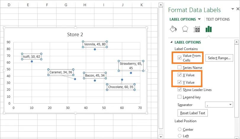
How to Print Labels From Excel - Lifewire To label a series in Excel, right-click the chart with the data series and choose Select Data. Under Legend Entries (Series), select the data series, then select Edit. Enter a name in the Series name field. How to add or move data labels in Excel chart? - ExtendOffice To add or move data labels in a chart, you can do as below steps: In Excel 2013 or 2016. 1. Click the chart to show the Chart Elements button . 2. Then click the Chart Elements, and check Data Labels, then you can click the arrow to choose an option about the data labels in the sub menu. See screenshot: In Excel 2010 or 2007. 1. click on the chart to show the Layout tab in the Chart Tools group. See screenshot: 2. Creating a chart with dynamic labels - Microsoft Excel 2016 1. Right-click on the chart and in the popup menu, select Add Data Labels and again Add Data Labels : 2. Do one of the following: For all labels: on the Format Data Labels pane, in the Label Options, in the Label Contains group, check Value From Cells and then choose cells:
Excel chart labels from cells. Automatically set chart axis labels from cell contents The (tick) labels occur at each > major tick along the axis. > > You can link the text of an axis title to a particular cell. Select the > axis title, press the equals key, and select the cell. > > This also works with the chart title, individual data labels, and text > boxes. > > - Jon > ------- > Jon Peltier, Microsoft Excel MVP Using the CONCAT function to create custom data labels for an Excel chart Use the chart skittle (the "+" sign to the right of the chart) to select Data Labels and select More Options to display the Data Labels task pane. Check the Value From Cells checkbox and select the cells containing the custom labels, cells C5 to C16 in this example. Excel Custom Chart Labels • My Online Training Hub Step 1: Select cells A26:D38 and insert a column Chart. Step 2: Select the Max series and plot it on the Secondary Axis: double click the Max series > Format Data Series > Secondary Axis: Step 3: Insert labels on the Max series: right-click series > Add Data Labels: How to Change Excel Chart Data Labels to Custom Values? You can change data labels and point them to different cells using this little trick. First add data labels to the chart (Layout Ribbon > Data Labels) Define the new data label values in a bunch of cells, like this: Now, click on any data label. This will select "all" data labels. Now click once again.
excel - Using VBA to create charts with data labels based on cell ... With x-axis data labels being set to the top row of headings (the blue range) With series labels being set according to the three group labels immediately to the left of the data. (the orange range) So far, all I've succeeded doing is the first one, based on this answer, resulting in the following code: Excel charts: add title, customize chart axis, legend and data labels ... Click the Chart Elements button, and select the Data Labels option. For example, this is how we can add labels to one of the data series in our Excel chart: For specific chart types, such as pie chart, you can also choose the labels location. For this, click the arrow next to Data Labels, and choose the option you want. How to Use Cell Values for Excel Chart Labels Select the chart, choose the "Chart Elements" option, click the "Data Labels" arrow, and then "More Options." Uncheck the "Value" box and check the "Value From Cells" box. Select cells C2:C6 to use for the data label range and then click the "OK" button. The values from these cells are now used for the chart data labels. How to link a cell to chart title/text box in Excel? 3. Go to the formula bar, and type the equal sign = into the formula bar, then select the cell you want to link to the chart title. See screenshot: 4. Press Enter key. Then you can see the selected cell is linked to chart title. Now when the cell A1 changes its contents, the chart title will automatically change.
Link a chart title, label, or text box to a worksheet cell On the Format tab, in the Current Selection group, click the arrow next to the Chart Elements box, and then click the chart element that you want to use. In the formula bar, type an equal sign ( = ). In the worksheet, select the cell that contains the data that you want to display in the title, label, or text box on the chart. Add or remove data labels in a chart - support.microsoft.com Click Label Options and under Label Contains, pick the options you want. Use cell values as data labels You can use cell values as data labels for your chart. Right-click the data series or data label to display more data for, and then click Format Data Labels. Click Label Options and under Label Contains, select the Values From Cells checkbox. Adding Data Labels To An Excel Chart | MyExcelOnline In our example below, I add a Data Label to a column chart and then I format the data label using CTRL+1. I then select to custom format the numbers so it shows the values as thousands by adding a comma , after each zero and then showing the work k by adding "k" Custom Data Labels with Colors and Symbols in Excel Charts - [How To] Step 3: Click inside the formula bar, Hit "=" button on keyboard and then click on the cell you want to link or type the address of that cell. In my case it is cell C2.Hit Enter key. Now the cell is connected to that data label. Repeat this process until all the cells are connected to each data label.
Add Custom Labels to x-y Scatter plot in Excel - DataScience Made Simple
How to add data labels from different column in an Excel chart? Please do as follows: 1. Right click the data series in the chart, and select Add Data Labels > Add Data Labels from the context menu to add... 2. Right click the data series, and select Format Data Labels from the context menu. 3. In the Format Data Labels pane, under Label Options tab, check the ...
Add Custom Labels to x-y Scatter plot in Excel - DataScience Made Simple
Create Dynamic Chart Data Labels with Slicers - Excel Campus You basically need to select a label series, then press the Value from Cells button in the Format Data Labels menu. Then select the range that contains the metrics for that series. Click to Enlarge Repeat this step for each series in the chart. If you are using Excel 2010 or earlier the chart will look like the following when you open the file.
Graphing with Excel - BIOLOGY FOR LIFE
Excel Charts - Option "Label contains value From cells" disappear How to calculate loan payments in Excel? Click here to reveal answer Use the PMT function: =PMT(5%/12,60,-25000) is for a $25,000 loan, 5% annual interest, 60 month loan.
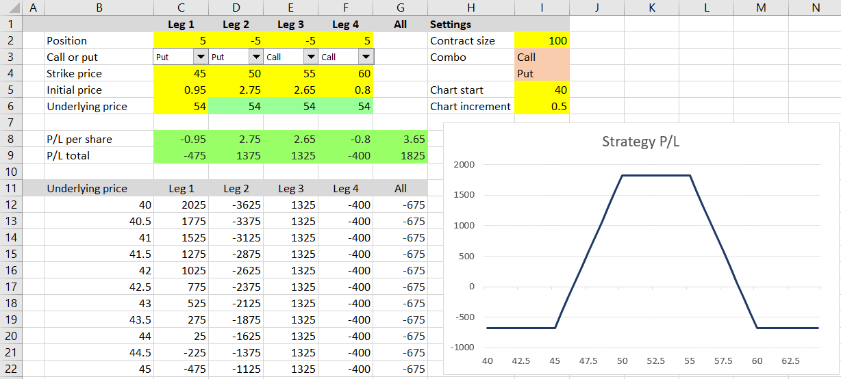
Drawing Option Payoff Diagrams in Excel - Macroption
Creating a chart with dynamic labels - Microsoft Excel 2016 1. Right-click on the chart and in the popup menu, select Add Data Labels and again Add Data Labels : 2. Do one of the following: For all labels: on the Format Data Labels pane, in the Label Options, in the Label Contains group, check Value From Cells and then choose cells:
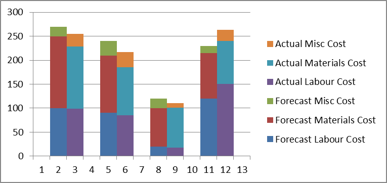
Step-by-step tutorial on creating clustered stacked column bar charts (for free) | Excel Help HQ
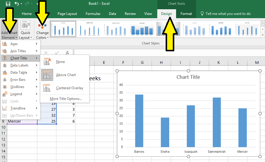
How to add or move data labels in Excel chart? - ExtendOffice To add or move data labels in a chart, you can do as below steps: In Excel 2013 or 2016. 1. Click the chart to show the Chart Elements button . 2. Then click the Chart Elements, and check Data Labels, then you can click the arrow to choose an option about the data labels in the sub menu. See screenshot: In Excel 2010 or 2007. 1. click on the chart to show the Layout tab in the Chart Tools group. See screenshot: 2.
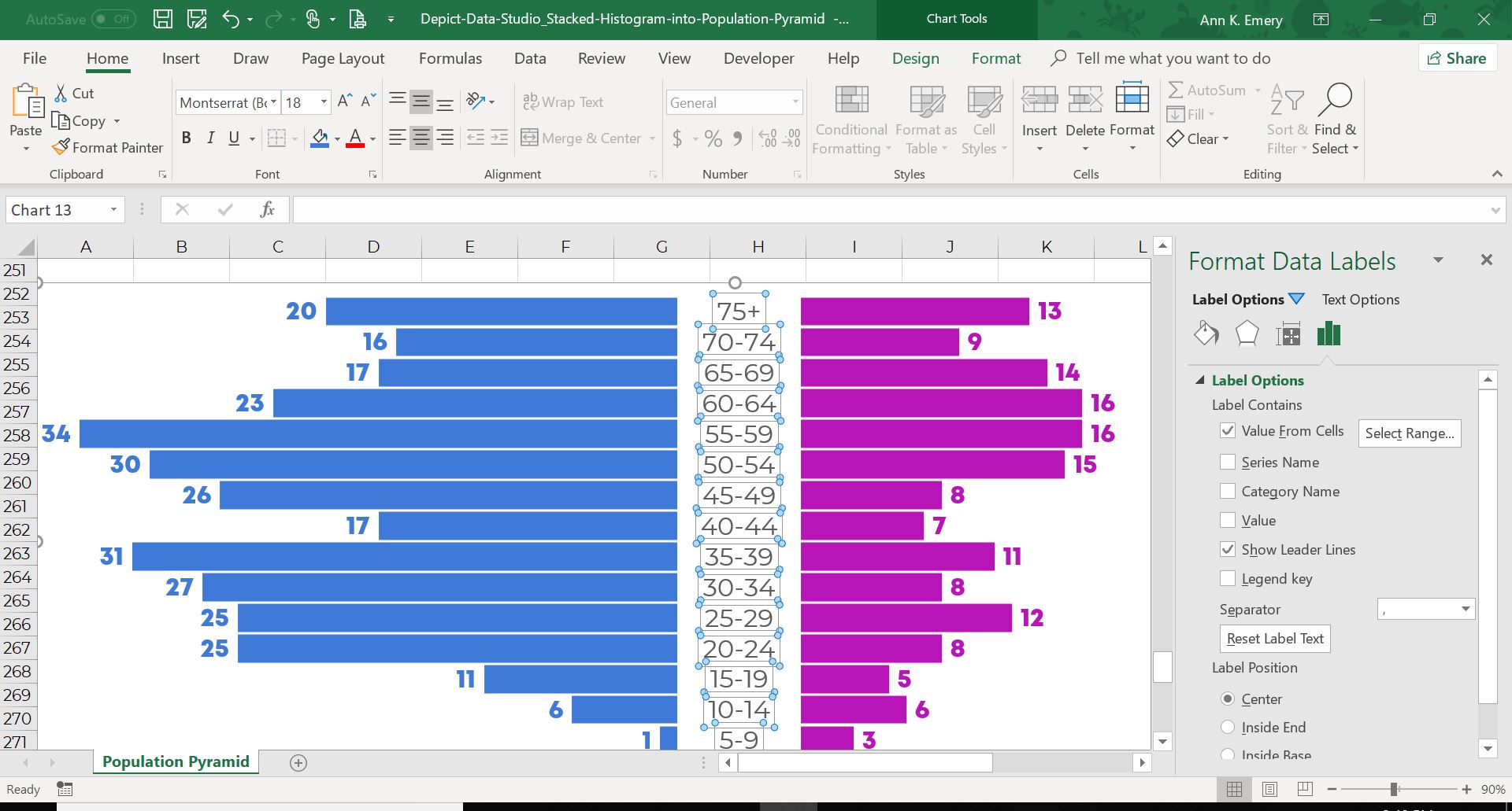
How to Visualize Age/Sex Patterns with Population Pyramids | Depict Data Studio
How to Print Labels From Excel - Lifewire To label a series in Excel, right-click the chart with the data series and choose Select Data. Under Legend Entries (Series), select the data series, then select Edit. Enter a name in the Series name field.

Excel Variance Charts: Making Awesome Actual vs Target Or Budget Graphs - How To ...
Debt Payoff Charts and Trackers
Post a Comment for "41 excel chart labels from cells"