45 excel pie chart don't show 0 labels

excel - How to not display labels in pie chart that are 0% - Stack Overflow Generate a new column with the following formula: =IF (B2=0,"",A2) Then right click on the labels and choose "Format Data Labels". Check "Value From Cells", choosing the column with the formula and percentage of the Label Options. Under Label Options -> Number -> Category, choose "Custom". Under Format Code, enter the following: I do not want to show data in chart that is "0" (zero) To access these options, select the chart and click: Chart Tools > Design > Select Data > Hidden and Empty Cells You can use these settings to control whether empty cells are shown as gaps or zeros on charts. With Line charts you can choose whether the line should connect to the next data point if a hidden or empty cell is found.

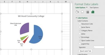
How to hide the zero percent labels in an Excel pie chart Remove the 0% in an Excel pie chart: Change the number format code of the labels 1) Select your chart and go to "Format Data Label": On Excel 2013: click on the "+" sign that appears on the top right of the chart and click on the arrow next to "Data Labels":

Excel pie chart don't show 0 labels

Hide Series Data Label if Value is Zero - Peltier Tech just go to .. data labels in charts ….select format data labels … in that select the option numbers … select custom .. give the format as "#,###;-#,###" then click add .. all the zeros will be ignored in the barchart……..It Works …. Juan Carlossays Monday, November 8, 2010 at 8:24 pm Hide zero values in chart labels- Excel charts WITHOUT zeros in labels ... 00:00 Stop zeros from showing in chart labels00:32 Trick to hiding the zeros from chart labels (only non zeros will appear as a label)00:50 Change the number... How to eliminate zero value labels in a pie chart - MrExcel Message Board My first thought was to include the Category Names next to the labels so that it would show 0% against the category and it would be clear what the 0% referred to. However you can hide the 0% using custom number formatting. Right click the label and select Format Data Labels. Then select the Number tab and then Custom from the Categories. Enter

Excel pie chart don't show 0 labels. Produce pie chart with Data Labels but not include the "Zero ... Answer. 1) if you only show the data values as the labels, format the data in the source table not to show zeros. For example, if your number format is 0.00 change it to. Then zero values will not show in the source data and also not in the labels. 2) if you want to show the data values and the category label, use a formula to create the labels ... How to Make a Scatter Plot in Excel (XY Chart) - Trump Excel A common scenario is where you want to plot X and Y values in a chart in Excel and show how the two values are related. This can be done by using a Scatter chart in Excel. For example, if you have the Height (X value) and Weight (Y Value) data for 20 students, you can plot this in a scatter chart and it will show you how the data is related. Top 10 ADVANCED Excel Charts and Graphs (Free Templates Download) Jun 30, 2017 · An Advanced Excel Chart or a Graph is a chart that has a specific use or presents data in a specific way for use. In Excel, an advanced chart can be created by using the basic charts which are already there in Excel, can be done from scratch, or using pre-made templates and add-ins. Display or hide zero values - support.microsoft.com If 0 is the result of (A2-A3), don't display 0 - display nothing (indicated by double quotes ""). If that's not true, display the result of A2-A3. If you don't want the cells blank but want to display something other than 0, put a dash "-" or other character between the double quotes. Hide zero values in a PivotTable report

How can I hide 0% value in data labels in an Excel Bar Chart Close out of your dialog box and your 0% labels should be gone. This works because Excel looks to your custom format to see how to format Postive;Negative;0 values. By leaving a blank after the final ; , Excel formats any 0 value as a blank. VBA Pie chart data labels in percentage, but need to exclude 0 ... - OzGrid However.. When the Pie charts are created based on my 6 columns, the data labels show as "0%" even though there is nothing in the cell. Is there a way to adjust below code so if the cell is blank/empty then when the charts are created, I don't have the "0%" labels in my charts How To Create A Pie Chart In Excel - PieProNation.com Create A Pie Chart From The Pivot Table. With everything we need in place, its time to create a pie chart using the pivot table you just built. Select any cell in your pivot table . Navigate to the Insert tab. Hit the Insert Pie or Doughnut Chart button. Under 2-D Pie, click Pie. How to hide zero data labels in chart in Excel? - ExtendOffice In the Format Data Labelsdialog, Click Numberin left pane, then selectCustom from the Categorylist box, and type #""into the Format Codetext box, and click Addbutton to add it to Typelist box. See screenshot: 3. Click Closebutton to close the dialog. Then you can see all zero data labels are hidden.

Pie Chart - Remove Zero Value Labels - Excel Help Forum The formulas in the source table can be written in such a way as to mask the zero or error values, but they still show up in the chart. Solution (Tested in Excel 2010.): 1. Right click on one of the chart "data labels" and choose "Format Data Labels." 2. Choose "Number" from the vertical menu on the left. 3. Excel – Create a Dynamic 12 Month Rolling Chart | Excelmate Jul 15, 2014 · To create a dynamic chart using this simple table we will need two named dynamic ranges – one for the data itself and one for the labels. Note that when working with charts you will need to create a separate dynamic range for each series as charts treat each series separately so you cannot create a single dynamic named range that includes all rows and columns. Pie Chart Data Callouts/Labels - Help with formatting the zero/blank ... I am working on some pie charts today that are giving me a problem with zero/blank values. I want my pie charts to only have Data Callouts for the slices that are relevant (not zero). Ex. My pie chart has 3 slices of apx. 30%, but when I use the Data Callouts or Labels buttons, a bunch of 0% values come up since I am using a bunch of variables. How to suppress 0 values in an Excel chart - TechRepublic The stacked bar and pie charts won't chart the 0 values, but the pie chart will display the category labels (as you can see in Figure E ). If this is a one-time charting task, just delete the...

How to make a pie chart in Excel

Google Sheets: Exclude X-Axis Labels If Y-Axis Values Are 0 or Blank Use the Query function. The easiest way to exclude x-axis labels from a chart if the corresponding y-axis values are 0 or blank is by simply hiding the rows containing the 0/null values. It's a manual method and you can use this on any chart types including Line, Column, Pie, Candlestick and so on. If there are a large number of records in ...

4.1 Choosing a Chart Type – Beginning Excel

How to Avoid overlapping data label values in Pie Chart In Reporting Services, when enabling data label in par charts, the position for data label only have two options: inside and outside. In your scenario, I recommend you to increase the size of the pie chart if you insist to choose the lable inside the pie chart as below: If you choose to "Enable 3D" in the chart area properties and choose to ...

r/excel - Pie Chart - I want to remove data labels if the value of the ... 1. level 1. tzim. 5 years ago. You should be able to click on the unwanted data labels and delete them individually. Otherwise you could exclude the zero value categories when you select the cells you want to use to populate the chart. 1. level 2. 13853211.

How To Make Pie Chart In Excel – Excel Examples

pie chart - Hide a range of data labels in 'pie of pie' in Excel ... Next select any slice from the main chart and hit CTRL+1 to bring up the Series Option window, here set the gap width to 0% (this will centre the main pie as much as possible) and set the second plot size to 5% (which is the minimum it will allow), and you have made your second pie invisible! Share answered Sep 7, 2015 at 1:02 Nobody 1

Highcharts简单条形图总数的百分比 - IT屋-程序员软件开发技术分享社区

Solved: Pie Chart Not Showing all Data Labels - Power BI Auto-suggest helps you quickly narrow down your search results by suggesting possible matches as you type.

How to make a pie chart in Excel

Rotate charts in Excel - spin bar, column, pie and line ... Jul 09, 2014 · I think 190 degrees will work fine for my pie chart. After being rotated my pie chart in Excel looks neat and well-arranged. Thus, you can see that it's quite easy to rotate an Excel chart to any angle till it looks the way you need. It's helpful for fine-tuning the layout of the labels or making the most important slices stand out. Rotate 3-D ...

Microsoft Excel Tutorials: Add Data Labels to a Pie Chart

Legend Entry Tricks in Excel Charts - Peltier Tech Feb 11, 2009 · In a pie chart, the legend labels are the category labels The easiest and most reliable way to set up data for a chart is to put category labels (or X values) in a column and (Y) values in the next column, then put a label in the cell above every value column (a pie chart has one value column) and leave the cell above the category labels blank.

How to Make a Pie Chart in Excel

Excel How to Hide Zero Values in Chart Label - YouTube Excel How to Hide Zero Values in Chart Label1. Go to your chart then right click on data label2. Select format data label3. Under Label Options, click on Num...

Best Charts in Excel and How To Use Them

How to Setup a Pie Chart with no Overlapping Labels - Telerik.com In Design view click on the chart series. The Properties Window will load the selected series properties. Change the DataPointLabelAlignment property to OutsideColumn. Set the value of the DataPointLabelOffset property to a value, providing enough offset from the pie, depending on the chart size (i.e. 30px).

How to Make a Pie Chart in Excel & Add Rich Data Labels to The Chart!

why are some data labels not showing in pie chart ... - Power BI Hi @Anonymous. Enlarge the chart, change the format setting as below. Details label->Label position: perfer outside, turn on "overflow text". For donut charts, you could refer to the following thread: How to show all detailed data labels of donut chart. Best Regards.

Hide Category & Value in Pie Chart if value is zero 1. Select the axis and press CTRL+1 (or right click and select "Format axis") 2. Go to "Number" tab. Select "Custom". 3. Specify the custom formatting code as #,##0;-#,##0;; 4. Press "Add" if you are using Excel 2007, otherwise press just OK. Any solution for Hiding Category also from chart if the value is zero and its display ...

31 How To Label Pie Charts In Excel - Labels Database 2020

Add or remove data labels in a chart - support.microsoft.com Click the data series or chart. To label one data point, after clicking the series, click that data point. In the upper right corner, next to the chart, click Add Chart Element > Data Labels. To change the location, click the arrow, and choose an option. If you want to show your data label inside a text bubble shape, click Data Callout.

Share :