41 conditional formatting pivot table row labels
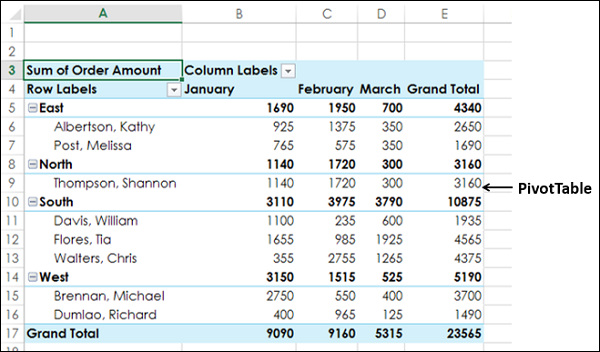
How to Apply Conditional Formatting to Pivot Tables So in this post I explain how to apply conditional formatting for pivot tables. 1. Select a cell in the Values area The first step is to select a cell in the Values area of the pivot table. If your pivot table has multiple fields in the Values area, select a cell for the field you want to apply the formatting to. 2. Apply Conditional Formatting Conditional Format Pivot Table Row - Chandoo.org Although the conditional formatting doesn't seem to extend across the row labels too. If I change this apply this option to include the label row. I receive the following error: cannot apply a conditional format to a range that has cells outside of a PivotTable data range.
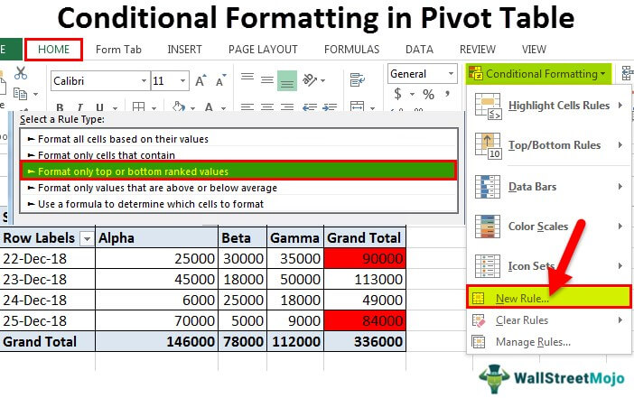
Conditional Formatting in Pivot Table (Example) | How To Apply? - EDUCBA Click on any cell in the pivot table > Go to the HOME tab > Click on Conditional Formatting option under Styles option > Click on Manage Rules option. It will open a Rules Manager dialog box. Click on the Edit Rule tab, as shown in the below screenshot. It will open the Editing Rule formatting window. Refer to the below screenshot.
Conditional formatting pivot table row labels
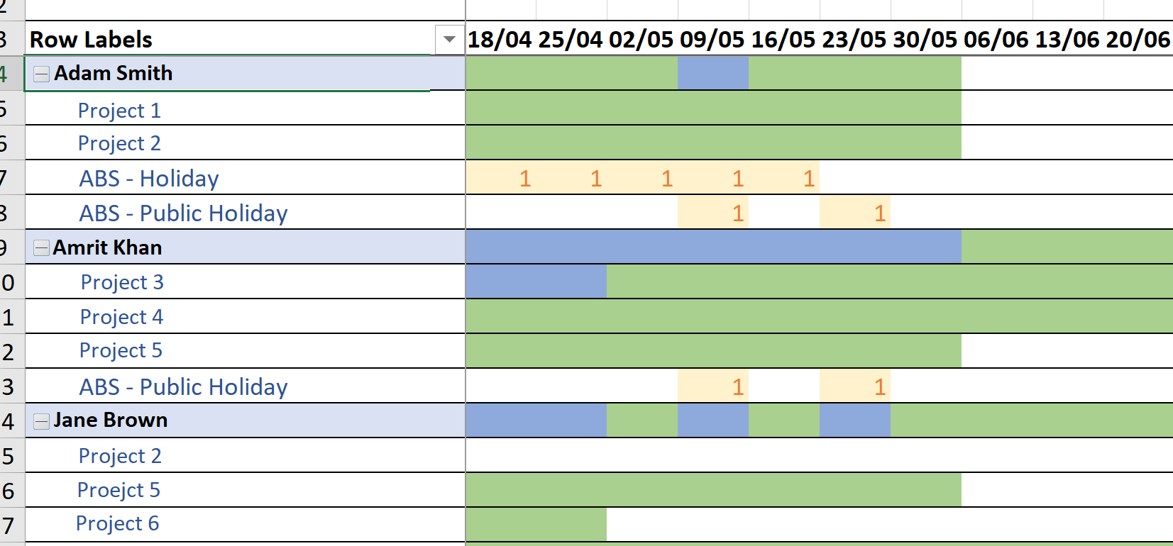
community.powerbi.com › t5 › Community-BlogConditional Formatting in Power BI Tables The Color Based on and Summarization drop downs auto-populate the same filed name you wish to apply conditional formatting on. In order to customize or change the fields for formatting, a drop down containing the table names and field names will appear and you can choose the required field according to your requirement. Conditional Formatting in Pivot Table - WallStreetMojo We must follow the steps to apply conditional formatting in the pivot table. First, we must select the data. Then, in the "Insert" Tab, click on "Pivot Tables." As a result, a dialog box appears. Next, we must insert the pivot table in a new worksheet by clicking "OK." Currently, a pivot table is blank. Next, we need to bring in the values. Format Pivot Table Labels Based on Date Range In the pivot table, remove any filters that have been applied - all the rows need to be visible before you apply the conditional formatting. Select all the dates in the Row Labels that you want to format. On the Ribbon, click the Home tab, and then in the Styles group, click Conditional Formatting.
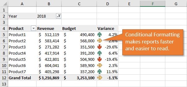
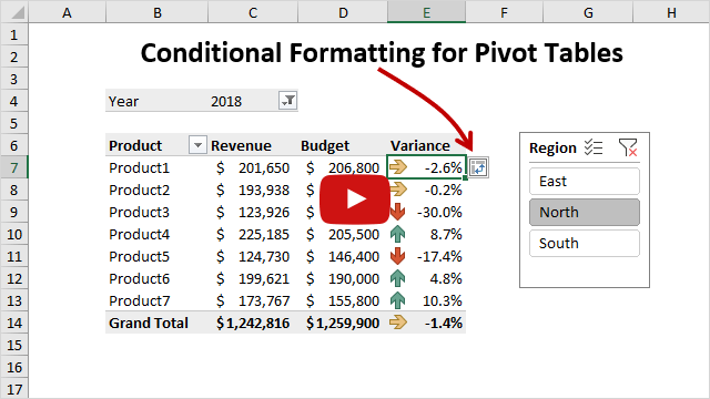
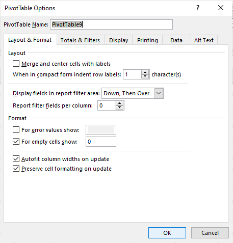
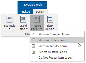
Conditional formatting pivot table row labels. Re-Apply Pivot Table Conditional Formatting - yoursumbuddy This method relies on all the conditional formatting you want to re-apply being in that first row labels cell. In cases where the conditional formatting might not apply to the leftmost row label, I've still applied it to that column, but modified the condition to check which column it's in. This function can be modified and called from a ... Overwrite pivot table conditional format based on row label As far as I know, using the one rule in the Conditional formatting, we can only format the cells with one color if the condition is true and if the same condition is false, the formatting of the cell will be blank and if both conditions are true, the formatting of cell depends on the highest ranking/priority of the rules in Conditional formatting. › blog › 50-things-you-can-do50 Things You Can Do With Excel Pivot Table | MyExcelOnline Jul 18, 2017 · STEP 1: Click on any variance value in the Pivot Table and go to Home > Conditional Formatting > Icon Sets > Directional. STEP 2: This will bring up the Apply Formatting Rule to dialogue box. Choose the 3rd option as this will apply the conditional format on all the values except the Subtotals. Your Pivot Table will look like this: Design the layout and format of a PivotTable To change the format of the PivotTable, you can apply a predefined style, banded rows, and conditional formatting. Windows Web Mac Changing the layout form of a PivotTable Change a PivotTable to compact, outline, or tabular form Change the way item labels are displayed in a layout form Change the field arrangement in a PivotTable
support.microsoft.com › en-us › officeUse Excel with earlier versions of Excel - support.microsoft.com The conditional formatting rules will not display the same results when you use these PivotTables in earlier versions of Excel. What it means Conditional formatting results you see in Excel 97-2003 PivotTable reports will not be the same as in PivotTable reports created in Excel 2007 and later. learn.microsoft.com › en-us › dotnetMicrosoft.Office.Interop.Excel Namespace | Microsoft Learn Object that enables single-click access to data analysis features such as formulas, conditional formatting, sparklines, tables, charts, and PivotTables. Range: Represents a cell, a row, a column, a selection of cells containing one or more contiguous blocks of cells, or a 3-D range. Ranges: A collection of Range objects. RecentFile Apply Conditional Formatting | Excel Pivot Table Tutorial Go to Home Tab → Styles → Conditional Formatting → New Rule. From rule to, select the third option. And, from "select a rule" type select "Format only top or bottom" ranked values. In edit rule description, enter 1 in the input box and from the drop-down menu select "each Column Group". Apply formatting you want. Click OK. spreadsheeto.com › pivot-tablesHow to Create a Pivot Table in Excel - Spreadsheeto To apply a conditional formatting rule to the entire Pivot Table, use the 2nd or 3rd options in the button that appears after using conditional formatting. Number formats Some data displays in an inherent logical way (e.g. currency starting with $ or £) .
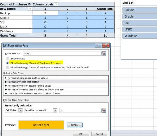
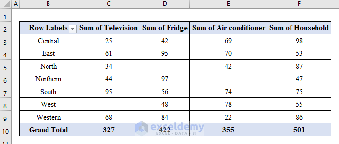
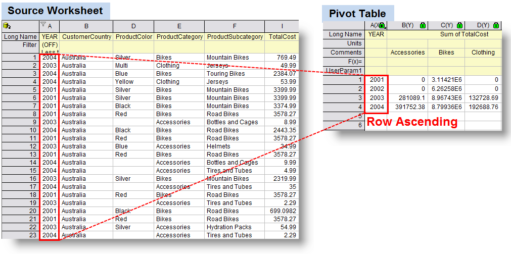
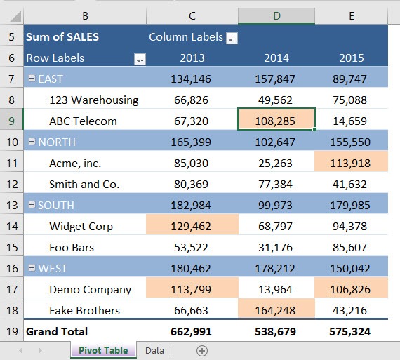
Conditional Formatting on Pivot Table row labels In srcFromPowerPivot sheet cell A is from powerpivot under row label comparing the dates in cell C (3 dates) and the condtional formatting doesnt work. In cell J it worked cos I dragged under value instead of row label. In the srcFromWorksheet it worked even though it is under rowlabel. Sheet3 is just a copy of powerpivot data. peltiertech.com › pivot-chart-formatting-changesPivot Chart Formatting Changes When Filtered - Peltier Tech Apr 07, 2014 · Here is Jon A’s original unfiltered pivot table on the left and mine (Jon P’s) on the right. His has six columns of values, mine has two. There are several pivot charts below each pivot table. The first chart under each pivot table has only default formatting applied: blue for series 1, orange for series two, gray for series three, etc. Pivot Table: Pivot table conditional formatting | Exceljet Select any cell in the data you wish to format and then choose "New rule" from the conditional formatting menu on the Home tab of the ribbon. At the top of the window, you will see setting for which cells to apply conditional formatting to. For the example shown, we want: "All cells showing sum of "sales values" for name and "date" Conditional formatting within fields pivot table Conditional formatting in a pivot table is tricky since the range of the pivot table can change when you filter or update the pivot table. ... Row Labels : Count of forecast: Customer 1 : Exports Americas: 11: Rest of the world: 2. Customer 2 . Exports Americas: 11. Rest of the world: 2 . Account Name: Year:
Maintaining Formatting when Refreshing PivotTables (Microsoft ...
Excel 2010 Conditional Formatting Pivot Table Row Labels Excel 2010 Conditional Formatting Pivot Table Row Labels. masuzi June 30, 2018 Uncategorized Leave a comment 14 Views. Conditional formatting for pivot tables how to apply conditional formatting conditional formatting for pivot tables conditional formatting for pivot tables.
Pivot Table Filter | CustomGuide
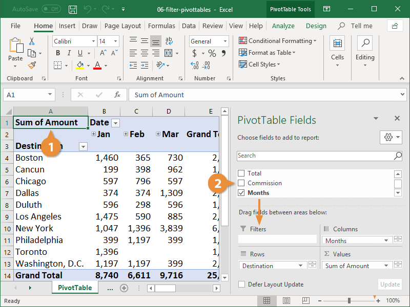
exceljet.net › pivot-table-tipsPivot Table Tips | Exceljet Your pivot table will now use it's own pivot cache and will not refresh with the other pivot table(s) in the workbook, or share the same field grouping. 19. Get rid of useless headings. The default layout for new pivot tables is the Compact layout. This layout will display "Row Labels" and "Column Labels" as headings in the pivot table.

Working with Pivot Tables | Excel library | Syncfusion
How to Apply Conditional Formatting in Pivot Table? (with Example) Currently, a pivot table is blank. Next, we need to bring in the values. Then, drag down the "Date" in the "Rows" Label, "Name" in the "Column," and "Sales" in "Values." As a result, the pivot table will look like the one below. To apply conditional formatting in the pivot table, first, we must select the column to format.
Formatting Tips for Pivot Tables - Goodly
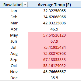
Format Pivot Table Labels Based on Date Range In the pivot table, remove any filters that have been applied - all the rows need to be visible before you apply the conditional formatting. Select all the dates in the Row Labels that you want to format. On the Ribbon, click the Home tab, and then in the Styles group, click Conditional Formatting.

Pivot Table Conditional Formatting
Conditional Formatting in Pivot Table - WallStreetMojo We must follow the steps to apply conditional formatting in the pivot table. First, we must select the data. Then, in the "Insert" Tab, click on "Pivot Tables." As a result, a dialog box appears. Next, we must insert the pivot table in a new worksheet by clicking "OK." Currently, a pivot table is blank. Next, we need to bring in the values.
How to Apply Conditional Formatting to Pivot Tables - Excel ...
community.powerbi.com › t5 › Community-BlogConditional Formatting in Power BI Tables The Color Based on and Summarization drop downs auto-populate the same filed name you wish to apply conditional formatting on. In order to customize or change the fields for formatting, a drop down containing the table names and field names will appear and you can choose the required field according to your requirement.

Format Pivot Table Labels Based on Date Range | Excel Pivot ...

Learn How to Apply Conditional Formatting in a Pivot Table ...

Pivot Table Conditional Formatting
Excel Pivot Tables - Sorting Data

Pivot Table: Pivot table conditional formatting | Exceljet

How to Apply Top/Bottom Rules In a Pivot Table- Conditional ...

Pivot Table Conditional Formatting Weekend Data Highlight

Excel Advanced Pivot Tables - Xelplus - Leila Gharani

How to Apply Conditional Formatting to Pivot Tables
How to Remove Blank Rows in Excel Pivot Table (4 Methods ...

In pivot tables how can I replace Row Labels with field names ...
Overwrite pivot table conditional format based on row label ...
Help Online - Origin Help - Pivot Table
How to Apply Conditional Formatting in Pivot Table? (with ...
Pivot Table Conditional Formatting in Excel - GeeksforGeeks

Conditional format a Pivot Table with the wizards ...
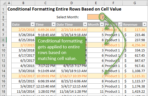
How to Apply Conditional Formatting to Rows Based on Cell ...
microsoft excel - How can I apply conditional formatting to ...
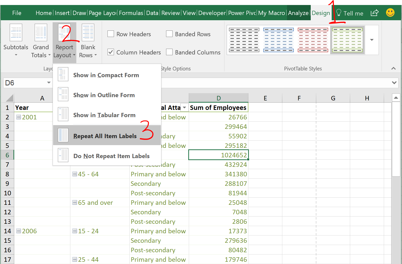
Repeat all item labels in Pivot Table (aka Fill in the blanks ...
Pivot Table Conditional Formatting | MyExcelOnline
How to Create a Pivot Table in Excel: Pivot Tables Explained

Pivot Table Grouping, Ungrouping And Conditional Formatting

How to Apply Conditional Formatting to a Pivot Table in Your ...
How to Apply Conditional Formatting to Pivot Tables - Excel ...
How to Remove Blanks in a Pivot Table in Excel (6 Ways ...
Change the PivotTable Layout | EarthCape Documentation

Unified Method of Pivot Table Formatting - yoursumbuddy

Pivot Table Conditional Formatting - Microsoft Community Hub
Conditional Formatting PivotTables • My Online Training Hub

vba - Pivot Table with Conditional Formatting: Where did my ...

Conditional Formatting in Pivot Table (Example) | How To Apply?
Excel: Apply Conditional Formatting to a Pivot Table - Excel ...
Pivot Table Conditional Formatting in Excel - GeeksforGeeks
Conditional Formatting in Excel - a Beginner's Guide

Customizing Pivot Table
Post a Comment for "41 conditional formatting pivot table row labels"